A Beginner’s Checklist for Evaluating a Climate Graph Online

To evaluate a climate graph online, do not begin by asking whether its line looks alarming or reassuring. Begin by identifying the source, variable, geographic coverage, time span, reference period and processing method. Then ask whether the accompanying claim is something the graph can actually establish.

No single online tool can certify an arbitrary graph as valid. Official tools can help you inspect data and attempt to reproduce a result, but methodological context still matters. A graph may plot genuine observations and remain misleading because it uses an unrepresentative interval, an unexplained baseline or a caption that goes beyond the evidence.

TLDR: Check these seven things first

1. Source: Who produced the data, and can you find the original dataset?
2. Variable: What was measured or estimated, in what units, and is it an absolute value or an anomaly?
3. Place: Does the graph cover one station, a country, an ocean region or the globe?
4. Time: What dates are included, and were the endpoints chosen for a defensible reason?
5. Baseline: If the graph shows anomalies, what reference period defines zero?
6. Processing: Are you looking at raw observations, adjusted data, a smoothed series, a fitted trend or a model projection?
7. Claim: Does the caption describe the evidence, or does it infer a cause or global conclusion that the graph alone cannot support?

1. Trace the graph to its original source

A logo or social-media account is not a data citation. Look for the organization, dataset name, version, download page and update date. If the image is cropped, search for distinctive wording from its title, axis labels or caption. The goal is to find the page where the variable and method are defined, not merely another copy of the picture.

Strong source pages normally provide metadata, downloadable values and methodological documentation. For example, the NOAA Global Temperature Anomalies graphing tool lets users choose variables, geography, dates, base periods and trend options, then download data in formats including CSV, JSON and XML. NASA’s GISTEMP v4 data page provides anomaly tables, gridded files, maps, source code and method information.

Failure to find an original source does not prove that a graph is false. It does mean you cannot yet verify how it was built, so confidence in precise claims should remain limited.

2. Identify exactly what the vertical axis measures

Read the axis label, units and legend together. “Temperature” could mean a station’s daily maximum, a monthly regional average, sea-surface temperature or an estimate combining land-surface air temperature with ocean measurements. These variables answer different questions. NOAA’s global product combines land-surface air temperature and sea-surface temperature, while NASA’s Land–Ocean Temperature Index is produced from land-station and ocean observations within its documented analysis framework.

Also determine whether the graph shows absolute temperature or temperature anomaly. An anomaly is the departure from a reference average for the same place and time of year. Anomalies are useful for broad comparisons because nearby locations can have very different absolute temperatures while exhibiting more comparable changes relative to their own normals.

3. Check the geographic coverage

A local record and a global average can both be accurate while showing different short-term patterns. Write down the graph’s actual domain: a named station, administrative region, latitude band, land area, ocean area or the whole globe. Geographic selections can legitimately change the plotted variability and calculated trend.

Be especially cautious when a caption moves between scales. A cold month at one station does not establish a global trend, and a global average does not tell you precisely what happened in every community. Regional questions may require regional evidence; the IPCC WGI Interactive Atlas provides assessed regional information with provenance and metadata for operations such as subsetting, gridding and index calculation.

4. Inspect the time span and endpoints

Climate describes average conditions over years or decades, while weather describes short-term atmospheric conditions. One month, one year or one endpoint cannot by itself establish a long-term climate trend.

Look at the first and last dates, then ask why they were selected. Starting at an unusually hot year can make later warming look smaller; starting at an unusually cool year can make it look larger. This does not mean every short interval is illegitimate. A short interval may be appropriate for a specific event or policy period, but it should not be presented as a complete account of a long-term trend.

When possible, expand the date range in the source tool. Compare the claimed interval with the full available record and with several nearby start dates. A conclusion that vanishes whenever the starting year moves slightly is probably sensitive to endpoint choice.

5. Record the anomaly baseline

If the axis says “anomaly,” “departure from average” or “change relative to,” find the reference period. NASA GISTEMP commonly reports anomalies relative to 1951–1980, while IPCC assessments commonly use 1850–1900 as an approximation of preindustrial global temperature.

Changing the baseline shifts the numerical anomaly values and the location of the zero line. By itself, it does not change the year-to-year differences or long-term trend. Two graphs can therefore show the same temperature evolution with different anomaly numbers.

Baseline choice still matters for interpretation. The World Meteorological Organization identifies 1991–2020 as the current standard 30-year normals period for many operational uses and retains 1961–1990 as a fixed historical reference for some long-term climate-change comparisons. A recent normal helps describe current conditions; a fixed historical period supports consistent comparison through time.

6. Separate observations, adjustments, smoothing and trends

Do not assume that every line represents individual measurements. It might show monthly observations, annual averages, a moving average, a statistical fit or a model projection. Check the legend and method notes for terms such as “five-year mean,” “LOESS,” “trend,” “ensemble mean” or “scenario.”

Smoothing suppresses some short-term variation so longer patterns are easier to see. A fitted trend summarizes change over a selected interval. Neither operation is automatically deceptive, but both must be labeled because they answer different questions from the unsmoothed observations. NOAA interfaces, for example, can display trend lines and smoothing methods including five-year means and LOESS; the fitted result depends partly on the selected interval.

Global temperature records are constructed estimates, not simple averages of every thermometer. Producers apply quality control, place observations on grids and estimate conditions in areas with sparse coverage. NASA also documents adjustments for non-climatic discontinuities such as station moves, equipment changes and changing observing conditions. Historical values can be updated when late reports, corrections, new observations or methodological improvements enter the analysis.

7. Look for uncertainty, not just a single line

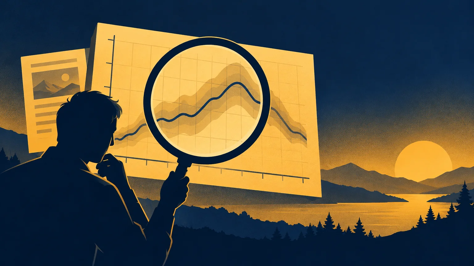
Uncertainty may appear as a shaded band, error bars, an ensemble range or a separate technical table. Its absence from the visible image does not necessarily mean the dataset ignores uncertainty, but you should look for it in the supporting documentation.

NASA provides a 200-member observational-uncertainty ensemble for GISTEMP v4 monthly historical anomalies covering 1880–2020. Its documentation highlights greater reasons for caution in areas such as polar regions and the Southern Ocean.

Uncertainty is not the same as ignorance. A range can be wide enough to affect an exact ranking while still supporting a clear long-term direction. Ask whether the uncertainty could materially change the specific conclusion being offered.

8. Test whether the caption follows from the graph

A graph can establish only what its variables and design permit. A line showing two quantities rising together demonstrates a visual association, not necessarily causation. Climate attribution draws on observations, physical understanding, theory, models and formal analyses rather than on one visual correlation.

Claims involving 1.5°C or 2°C need particular care. Check the baseline—normally 1850–1900 in IPCC usage—and distinguish a single year’s anomaly from an assessed multi-year global-warming level. Those are related measurements, but they are not interchangeable.

Question	Reassuring sign	Reason to investigate
Where did the data come from?	Named dataset, version and original download page	Only a screenshot, repost or vague institutional logo
What is plotted?	Variable, units and anomaly definition are explicit	Axis label is missing or uses an undefined “change”
What area is covered?	Station, region or global domain is stated	A local series is described as global evidence
Why these dates?	Interval matches the question and longer context is available	A narrow range begins or ends at an unexplained extreme
What processing occurred?	Smoothing, adjustments and trend methods are documented	A clean curve appears with no method or underlying values
How certain is it?	Uncertainty or limitations are available	Tiny differences are treated as exact or decisive
What does the caption claim?	Wording matches the variable and scale	Correlation is presented as causal attribution

A quick verification workflow

1. Save the image or URL before it changes, and note the claim attached to it.
2. Locate the original dataset and methodological page.
3. Write down the variable, units, area, dates, baseline and processing method.
4. Download the values or recreate the selection in an official tool when possible.
5. Change one choice at a time—such as the date range, region or smoothing option—and observe what changes.
6. Compare the long-term pattern with another established analysis that uses a different method.
7. Rewrite the claim in narrow, literal language. If the graph does not support that sentence, do not share the stronger version.

Independent global temperature analyses from NASA, NOAA, Hadley/CRU and Berkeley Earth use different methods but closely agree on the long-term global warming pattern. Differences can be more consequential in early sea-surface records and high-latitude regions, so comparison is most useful when it focuses on both agreement and known areas of uncertainty.

If the graph is part of a broader post or argument, continue with the publication’s guide to fact-checking a climate claim before sharing it. That next step checks whether quotations, headlines and contextual claims accurately represent the underlying evidence.

The practical takeaway

A graph earns confidence through traceability. You should be able to identify what was measured, where and when it was measured, how the values were processed, what baseline was used and how uncertainty affects the conclusion. Reproducing the exact image is helpful, but understanding those choices is more important than making the lines look identical.

When time is limited, prioritize three questions: Can I find the original data? Do I understand both axes? Does the caption claim more than the graph shows? Those checks will not settle every technical dispute, but they catch many of the most common ways an otherwise real climate dataset becomes a misleading online argument.

References

1. Global Temperature Anomalies – Graphing Tool | NOAA Climate.gov
2. Data.GISS: GISS Surface Temperature Analysis (GISTEMP v4)
3. IPCC WGI Interactive Atlas
4. NOAAGlobalTemp | National Centers for Environmental Information (NCEI)
5. Data.GISS: GISTEMP — Frequently Asked Questions
6. Weather
7. Climate at a Glance | National Time Series | National Centers for Environmental Information (NCEI)
8. IPCC AR6 Working Group 1: Summary for Policymakers | Climate Change 2021: The Physical Science Basis
9. WMO Climatological Normals
10. Updated 30-year reference period reflects changing climate
11. Climate change: global temperature | NOAA Climate.gov
12. data.giss.nasa.gov
13. Data.GISS: GISTEMP Uncertainty Analysis: Observational Uncertainty Ensemble
14. Approved Version  Summary for Policymakers  IPCC AR6 WGI
15. The Raw Truth on Global Temperature Records – NASA Science